Sparse Networks with Overlapping Communities (SNOC) package: demo_overlappingcommunity
This Matlab script finds overlapping communities in a network of political blogs, using the wrapper function overlapping_community_detection.m. For a full analysis of this dataset, see the Matlab demo demo_polblogs.m.
For downloading the package and information on installation, visit the SNOC webpage.
Reference:
- A. Todeschini, X. Miscouridou and F. Caron (2017) Exchangeable Random Measures for Sparse and Modular Graphs with Overlapping Communities. arXiv:1602.02114.
Authors:
- A. Todeschini, Inria
- X. Miscouridou, University of Oxford
- F. Caron, University of Oxford
Tested on Matlab R2016a. Requires the statistics toolbox.
Last Modified: 07/11/2017
Contents
close all
clear all

% Add path
addpath ./GGP/ ./CGGP/ ./utils/
Load network of political blogs
Data can be downloaded from here.
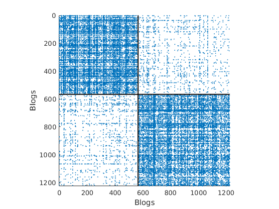
load ./data/polblogs/polblogs.mat

titlenetwork = 'Political blogosphere Feb. 2005';
name = 'polblogs';
labels = {'Blogs', 'Blogs'};
groupfield = 'name'; % meta field displayed for group plot

% Transform the graph to obtain a simple graph
G = Problem.A | Problem.A'; % make undirected graph
G = logical(G-diag(diag(G))); % remove self edges (#3)

% Collect metadata
meta.name = cellstr(Problem.aux.nodename);
meta.source = cellstr(Problem.aux.nodesource);
meta.isright = logical(Problem.aux.nodevalue);
meta.degree = num2cell(full(sum(G,2)));
meta.groups = zeros(size(meta.isright));
meta.groups(~meta.isright) = 1;
meta.groups(meta.isright) = 2;
color_groups = [0 0 .8; .8 0 0];
label_groups = {'Left', 'Right'};
fn = fieldnames(meta);

% Remove nodes with no edge (#266)
ind = any(G);
G = G(ind, ind);
for i=1:length(fn)
    meta.(fn{i}) = meta.(fn{i})(ind);
end

% Plot adjacency matrix (sorted)
figure('name', 'Adjacency matrix (sorted by ground truth political leaning)')
spy(G);
xlabel(labels{2})
ylabel(labels{1})
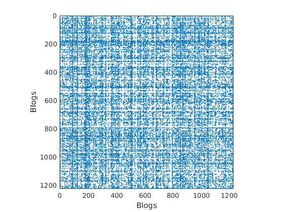
% Shuffle nodes: irrelevant due to exchangeability, just to check we do not cheat!
ind = randperm(size(G,1));
G = G(ind, ind);
for i=1:length(fn)
    meta.(fn{i}) = meta.(fn{i})(ind);
end

% Plot adjacency matrix (unsorted)
figure('name', 'Adjacency matrix (unsorted)')
spy(G);
xlabel(labels{2})
ylabel(labels{1})
Find overlapping communities
p = 2; % Number of communities
niter = 20000; % Number of iterations
[degree_correction, community_affiliation, community_detection] = overlapping_community_detection(G, p, niter);
-----------------------------------
Start initialisation of the MCMC algorithm for CGGP
-----------------------------------
End initialisation
-----------------------------------
-----------------------------------
Start MCMC for CGGP graphs
Nb of nodes: 1224 - Nb of edges: 16715 (0 missing)
Nb of chains: 1 - Nb of iterations: 20000
Nb of parallel workers: 1
Estimated computation time: 0 hour(s) 2 minute(s)
Estimated end of computation: 08-Nov-2017 18:01:19
-----------------------------------
 Markov chain 1/1
-----------------------------------
i=2000 alp=669.22 sig=-0.255 tau=1.98 a=0.23 0.18 b=0.46 0.39 w*=0.56 0.36 b2=0.90 0.78 alp2=562.24 rhmc=0.63 rhyp=0.30 eps=0.025 rwsd=0.049
i=4000 alp=1604.00 sig=-0.450 tau=3.68 a=0.20 0.15 b=0.39 0.27 w*=0.50 0.41 b2=1.42 1.01 alp2=892.66 rhmc=0.70 rhyp=0.25 eps=0.04 rwsd=0.058
i=6000 alp=1718.53 sig=-0.453 tau=3.48 a=0.18 0.14 b=0.36 0.31 w*=0.47 0.39 b2=1.24 1.06 alp2=977.03 rhmc=0.56 rhyp=0.22 eps=0.025 rwsd=0.056
i=8000 alp=1687.01 sig=-0.450 tau=3.93 a=0.18 0.15 b=0.32 0.29 w*=0.47 0.39 b2=1.24 1.12 alp2=911.42 rhmc=0.78 rhyp=0.23 eps=0.025 rwsd=0.056
i=10000 alp=1799.57 sig=-0.468 tau=3.91 a=0.16 0.13 b=0.29 0.24 w*=0.46 0.41 b2=1.13 0.92 alp2=950.12 rhmc=0.79 rhyp=0.23 eps=0.025 rwsd=0.056
i=12000 alp=2018.04 sig=-0.458 tau=4.47 a=0.16 0.13 b=0.28 0.20 w*=0.50 0.49 b2=1.24 0.89 alp2=1016.53 rhmc=0.78 rhyp=0.23 eps=0.025 rwsd=0.056
i=14000 alp=1999.09 sig=-0.459 tau=4.66 a=0.15 0.12 b=0.18 0.19 w*=0.46 0.42 b2=0.84 0.88 alp2=985.82 rhmc=0.78 rhyp=0.23 eps=0.025 rwsd=0.056
i=16000 alp=2012.28 sig=-0.491 tau=3.99 a=0.14 0.12 b=0.23 0.22 w*=0.55 0.37 b2=0.92 0.88 alp2=1019.78 rhmc=0.78 rhyp=0.23 eps=0.025 rwsd=0.056
i=18000 alp=1805.01 sig=-0.456 tau=3.90 a=0.14 0.12 b=0.28 0.24 w*=0.50 0.41 b2=1.11 0.95 alp2=970.22 rhmc=0.78 rhyp=0.23 eps=0.025 rwsd=0.056
i=20000 alp=1790.90 sig=-0.486 tau=3.11 a=0.13 0.12 b=0.27 0.33 w*=0.56 0.42 b2=0.84 1.03 alp2=1032.27 rhmc=0.77 rhyp=0.24 eps=0.025 rwsd=0.056
-----------------------------------
End MCMC
Computation time: 0 hour(s) 1 minute(s)
-----------------------------------
-----------------------------------
Start parameters estimation for CGGP graphs: 500 samples
Estimated end of computation: 08-Nov-2017 18:01:33 (0.0 hours)
|---------------------------------|
|*********************************|
End parameters estimation for CGGP graphs
Computation time: 0.0 hours
-----------------------------------
Some plots
% Identify each feature as liberal or conservative using ground truth
% (This step would normally require a human interpretation of the features)
[~, ind_features] = sort(median(community_affiliation(meta.isright,:), 1)./median(community_affiliation, 1));
featnames = {'Liberal', 'Conservative'}; % Name of the interpreted features

% Print classification performance with ground truth
[confmat] = print_classif(fullfile('./', ['classif_' num2str(p) 'f.txt']), ...
    community_detection, meta.groups, ind_features, label_groups);
Classification performance
==========================
Confusion matrix (counts)
-------------------------
Group        : Feat 1 Feat 2 | Total
Left         :    543     45 |   588
Right        :     23    613 |   636
Total        :    566    658 |  1224
-------------------------
Confusion matrix (%)
-------------------------
Group        : Feat 1 Feat 2 | Total
Left         :  44.36   3.68 | 48.04
Right        :   1.88  50.08 | 51.96
Total        :  46.24  53.76 |100.00
-------------------------
Group assignments of features
-------------------------
Feat 1: Left
Feat 2: Right
-------------------------
Accuracy = 94.44
Error = 5.56
==========================
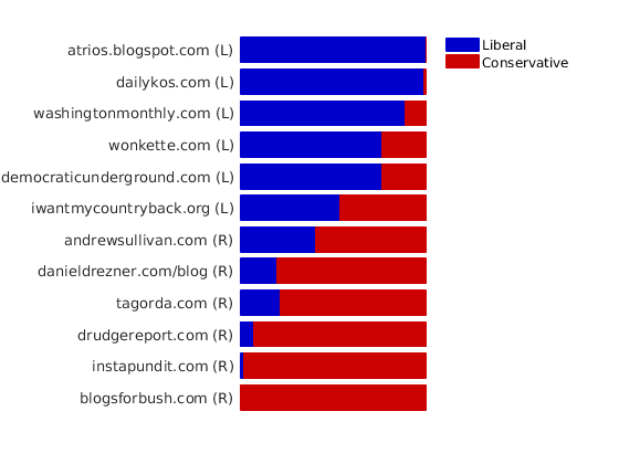
% Plot levels of affiliation to each community for a subset of blogs
color = [0 0 .8; .8 0 0];
names = {'blogsforbush.com'
    'instapundit.com'
    'drudgereport.com'
    'tagorda.com'
    'danieldrezner.com/blog'
    'andrewsullivan.com'
    'iwantmycountryback.org'
    'democraticunderground.com'
    'wonkette.com'
    'washingtonmonthly.com'
    'dailykos.com'
    'atrios.blogspot.com'};
ind = zeros(size(names,1),1);
lab = cell(size(names,1), 1);
for i=1:size(names,1)
    ind(i) = find(strcmp(meta.name, names{i}) & strcmp(meta.name, names{i,1}));
    lab{i} = sprintf('%s (%s)', names{i}, label_groups{meta.groups(ind(i))}(1));
end
plot_nodesfeatures(community_affiliation, ind, ind_features, lab, featnames, color);
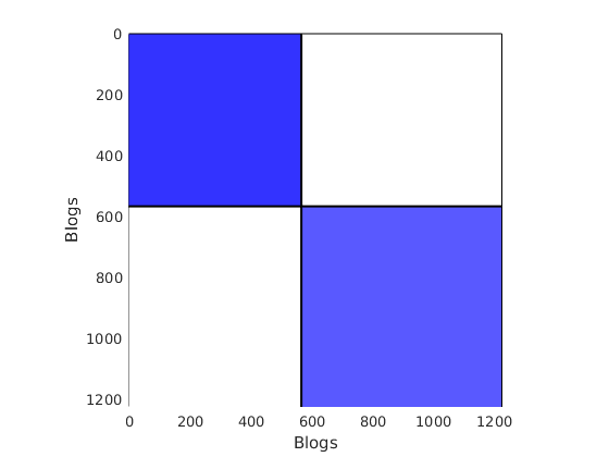
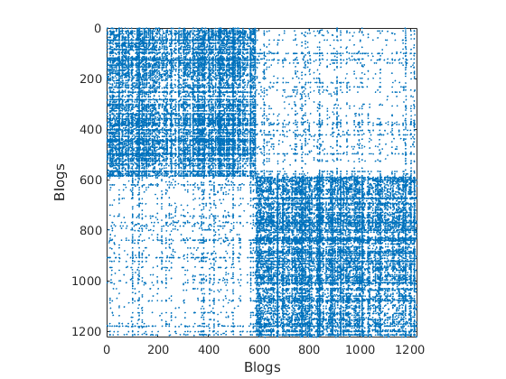
% Plot the graph by clustering the nodes by community with maximum level of affiliation to see block structure
plot_sortedgraph(G, community_detection, community_detection, ind_features, labels);