Sparse Networks with Overlapping Communities (SNetOC) package: demo_polblogs

This Matlab script performs posterior inference on a network of political blogs to find latent overlapping communities, using a Bayesian nonparametric approach.

For downloading the package and information on installation, visit the SNetOC webpage.

Reference:

A. Todeschini, X. Miscouridou and F. Caron (2017) Exchangeable Random Measures for Sparse and Modular Graphs with Overlapping Communities. arXiv:1602.02114.

Authors:

A. Todeschini, Inria
X. Miscouridou, University of Oxford
F. Caron, University of Oxford

Tested on Matlab R2016a. Requires the Statistics toolbox.

Last Modified: 10/2017

General settings
Load network of political blogs
Posterior Inference using Markov chain Monte Carlo and point estimation
Plots

General settings

clear
close all
tstart = clock; % Starting time

istest = true; % enable testing mode: quick run with smaller nb of iterations

In test mode, a smaller number of iterations is run. Although the sampler clearly has not converged yet, the method already recovers well the ground truth communities. To reproduce the results of the paper, set this value to false.

root = '.';
if istest
    outpath = fullfile(root, 'results', 'demo_polblogs', 'test');
else
    outpath = fullfile(root, 'results', 'demo_polblogs', date);
end

if ~isdir(outpath)
    mkdir(outpath);
end

% Add path
addpath ./GGP/ ./CGGP/ ./utils/

set(0, 'DefaultAxesFontSize', 14)

% Set the seed
rng default

Load network of political blogs

Data can be downloaded from here.

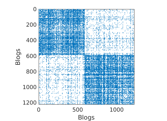
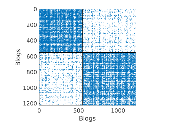
load ./data/polblogs/polblogs.mat

titlenetwork = 'Political blogosphere Feb. 2005';
name = 'polblogs';
labels = {'Blogs', 'Blogs'};
groupfield = 'name'; % meta field displayed for group plot

% Transform the graph to obtain a simple graph
G = Problem.A | Problem.A'; % make undirected graph
G = logical(G-diag(diag(G))); % remove self edges (#3)

% Collect metadata
meta.name = cellstr(Problem.aux.nodename);
meta.source = cellstr(Problem.aux.nodesource);
meta.isright = logical(Problem.aux.nodevalue);
meta.degree = num2cell(full(sum(G,2)));
meta.groups = zeros(size(meta.isright));
meta.groups(~meta.isright) = 1;
meta.groups(meta.isright) = 2;
color_groups = [0 0 .8; .8 0 0];
label_groups = {'Left', 'Right'};
fn = fieldnames(meta);

% Remove nodes with no edge (#266)
ind = any(G);
G = G(ind, ind);
for i=1:length(fn)
    meta.(fn{i}) = meta.(fn{i})(ind);
end

% Plot adjacency matrix (sorted)
figure('name', 'Adjacency matrix (sorted by ground truth political leaning)')
spy(G);
xlabel(labels{2})
ylabel(labels{1})

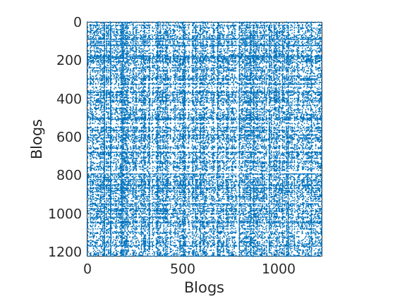
% Shuffle nodes: irrelevant due to exchangeability, just to check we do not cheat!
ind = randperm(size(G,1));
G = G(ind, ind);
for i=1:length(fn)
    meta.(fn{i}) = meta.(fn{i})(ind);
end

% Plot adjacency matrix (unsorted)
figure('name', 'Adjacency matrix (unsorted)')
spy(G);
xlabel(labels{2})
ylabel(labels{1})

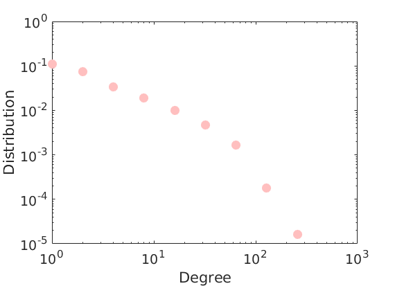
% Plot degree distribution
figure('name', 'Empirical degree distribution')
hdeg = plot_degree(G);
set(hdeg, 'markersize', 10, 'marker', 'o','markeredgecolor', 'none', 'markerfacecolor', [1, .75, .75]);

Posterior Inference using Markov chain Monte Carlo and point estimation

Users needs to start the parallel pool by using the command parpool to run multiple chains in parallel.

% Define the parameters of the prior
p = 2; % Number of commmunities
objprior =  graphmodel('CGGP', p); % CGGP graph model with p communities

% Define parameters of the MCMC sampler
nchains = 3;
if istest
    niterinit = 1000;
    niter = 10000;
    nsamples = 100;
else
    niterinit = 10000;
    niter = 200000;
    nsamples = 500;
end
nburn = floor(niter/2);

thin = ceil((niter-nburn)/nsamples);
verbose = true;

% Create the graphMCMC object
objmcmc = graphmcmc(objprior, niter, nburn, thin, nchains);

% Run initialisation
init = graphinit(objmcmc, G, niterinit);

-----------------------------------
Start initialisation of the MCMC algorithm for CGGP
-----------------------------------
End initialisation
-----------------------------------

% Run MCMC sampler
objmcmc = graphmcmcsamples(objmcmc, G, verbose, init);

-----------------------------------
Start MCMC for CGGP graphs
Nb of nodes: 1224 - Nb of edges: 16715 (0 missing)
Nb of chains: 3 - Nb of iterations: 10000
Nb of parallel workers: 1
Estimated computation time: 0 hour(s) 2 minute(s)
Estimated end of computation: 08-Nov-2017 18:03:33 
-----------------------------------
 Markov chain 1/3 
-----------------------------------
i=2000 alp=853.49 sig=-0.318 tau=2.23 a=0.22 0.20 b=0.41 0.51 w*=0.52 0.40 b2=0.91 1.13 alp2=661.59 rhmc=0.68 rhyp=0.32 eps=0.028 rwsd=0.054
i=4000 alp=1625.62 sig=-0.482 tau=3.37 a=0.20 0.16 b=0.40 0.31 w*=0.46 0.50 b2=1.35 1.04 alp2=905.44 rhmc=0.72 rhyp=0.23 eps=0.022 rwsd=0.054
i=6000 alp=1787.89 sig=-0.462 tau=4.23 a=0.17 0.14 b=0.27 0.23 w*=0.51 0.52 b2=1.14 0.99 alp2=917.85 rhmc=0.83 rhyp=0.24 eps=0.022 rwsd=0.054
i=8000 alp=1899.11 sig=-0.474 tau=4.23 a=0.16 0.14 b=0.27 0.26 w*=0.56 0.43 b2=1.14 1.11 alp2=958.50 rhmc=0.83 rhyp=0.26 eps=0.022 rwsd=0.054
i=10000 alp=1988.12 sig=-0.496 tau=3.79 a=0.15 0.13 b=0.30 0.32 w*=0.47 0.36 b2=1.13 1.22 alp2=1026.23 rhmc=0.82 rhyp=0.23 eps=0.022 rwsd=0.054
-----------------------------------
 Markov chain 2/3 
-----------------------------------
i=2000 alp=704.00 sig=-0.235 tau=2.52 a=0.21 0.21 b=0.44 0.32 w*=0.50 0.55 b2=1.11 0.80 alp2=566.75 rhmc=0.67 rhyp=0.32 eps=0.024 rwsd=0.054
i=4000 alp=1259.23 sig=-0.379 tau=3.55 a=0.16 0.17 b=0.28 0.25 w*=0.41 0.56 b2=1.00 0.87 alp2=779.78 rhmc=0.77 rhyp=0.23 eps=0.022 rwsd=0.052
i=6000 alp=1958.77 sig=-0.467 tau=4.44 a=0.14 0.18 b=0.21 0.28 w*=0.43 0.47 b2=0.92 1.23 alp2=976.18 rhmc=0.82 rhyp=0.25 eps=0.022 rwsd=0.052
i=8000 alp=2059.08 sig=-0.505 tau=4.33 a=0.15 0.17 b=0.27 0.31 w*=0.46 0.42 b2=1.16 1.32 alp2=983.15 rhmc=0.82 rhyp=0.25 eps=0.022 rwsd=0.052
i=10000 alp=1942.87 sig=-0.493 tau=3.97 a=0.15 0.17 b=0.31 0.23 w*=0.34 0.54 b2=1.21 0.90 alp2=984.37 rhmc=0.81 rhyp=0.26 eps=0.022 rwsd=0.052
-----------------------------------
 Markov chain 3/3 
-----------------------------------
i=2000 alp=444.90 sig=-0.129 tau=1.93 a=0.22 0.23 b=0.19 0.32 w*=0.49 0.45 b2=0.37 0.61 alp2=408.74 rhmc=0.68 rhyp=0.32 eps=0.038 rwsd=0.052
i=4000 alp=1226.02 sig=-0.358 tau=4.20 a=0.19 0.17 b=0.20 0.21 w*=0.46 0.40 b2=0.86 0.89 alp2=733.18 rhmc=0.70 rhyp=0.24 eps=0.021 rwsd=0.053
i=6000 alp=1367.94 sig=-0.376 tau=4.33 a=0.17 0.15 b=0.20 0.22 w*=0.52 0.39 b2=0.88 0.94 alp2=788.40 rhmc=0.84 rhyp=0.24 eps=0.021 rwsd=0.053
i=8000 alp=2250.42 sig=-0.499 tau=5.26 a=0.18 0.14 b=0.24 0.20 w*=0.48 0.38 b2=1.26 1.07 alp2=981.84 rhmc=0.84 rhyp=0.25 eps=0.021 rwsd=0.053
i=10000 alp=2427.51 sig=-0.534 tau=5.11 a=0.16 0.15 b=0.20 0.25 w*=0.47 0.45 b2=1.04 1.26 alp2=1015.77 rhmc=0.84 rhyp=0.23 eps=0.021 rwsd=0.053
-----------------------------------
End MCMC
Computation time: 0 hour(s) 2 minute(s)
-----------------------------------

% Print summary in text file
print_summary(['summary_' num2str(p) 'f.txt'], titlenetwork, G, niter, nburn, nchains, thin, p, outpath, tstart)

% Point estimation of the model parameters
[estimates, C_st] = graphest(objmcmc);

% Save workspace
save(fullfile(outpath, ['workspace_' num2str(p) 'f.mat']))

-----------------------------------
Start parameters estimation for CGGP graphs: 300 samples
Estimated end of computation: 08-Nov-2017 18:03:38 (0.0 hours)
|---------------------------------|
|*********************************|
End parameters estimation for CGGP graphs
Computation time: 0.0 hours
-----------------------------------

Plots

prefix = sprintf('%s_%df_', name, p);
suffix = '';

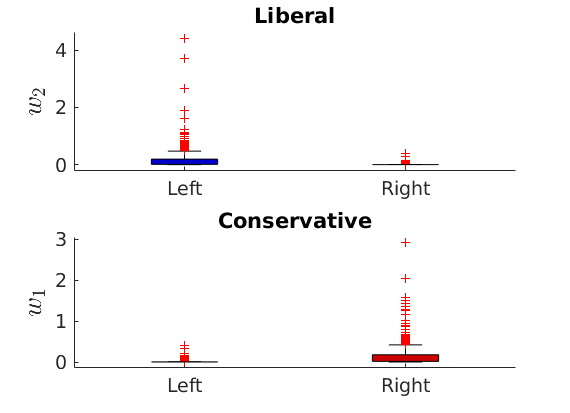
% Identify each feature to left/right wing using ground truth
% (This step would normally require a human interpretation of the features)
[~, ind_features] = sort(median(estimates.w(meta.isright,:), 1)./median(estimates.w, 1));
featnames = {'Liberal', 'Conservative'};

% Print classification performance with ground truth
[~, nodefeat] = max(estimates.w, [],2); % Assign each node to the feature with highest weight
[confmat] = print_classif(fullfile(outpath, ['classif_' num2str(p) 'f.txt']), ...
    nodefeat, meta.groups, ind_features, label_groups);

Classification performance
==========================
Confusion matrix (counts)
-------------------------
Group        : Feat 1 Feat 2 | Total
Left         :    530     58 |   588
Right        :     22    614 |   636
Total        :    552    672 |  1224
-------------------------
Confusion matrix (%)
-------------------------
Group        : Feat 1 Feat 2 | Total
Left         :  43.30   4.74 | 48.04
Right        :   1.80  50.16 | 51.96
Total        :  45.10  54.90 |100.00
-------------------------
Group assignments of features
-------------------------
Feat 1: Left
Feat 2: Right
-------------------------
Accuracy = 93.46
Error = 6.54
==========================

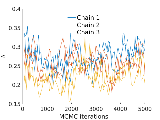
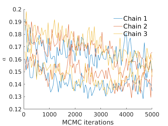
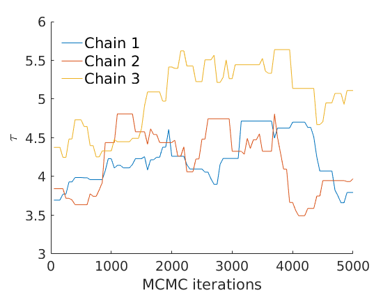
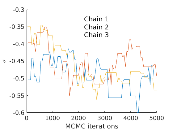
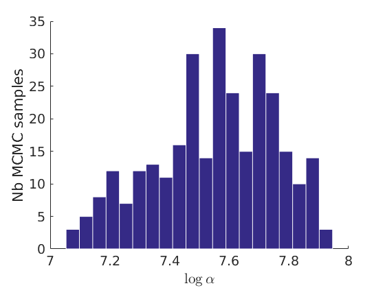
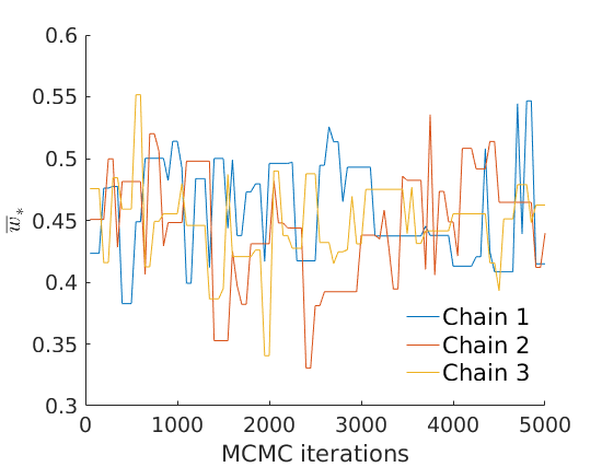
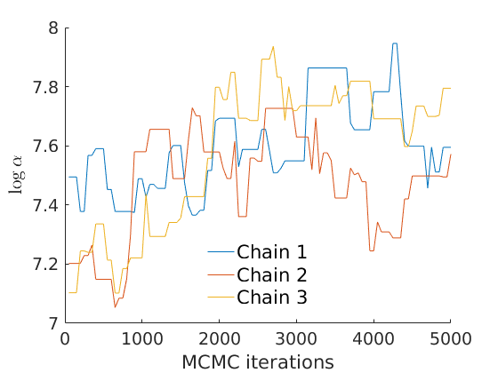
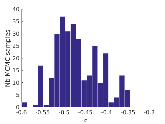
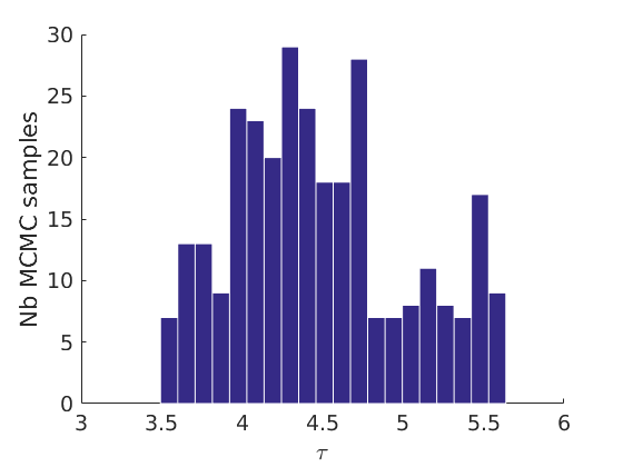
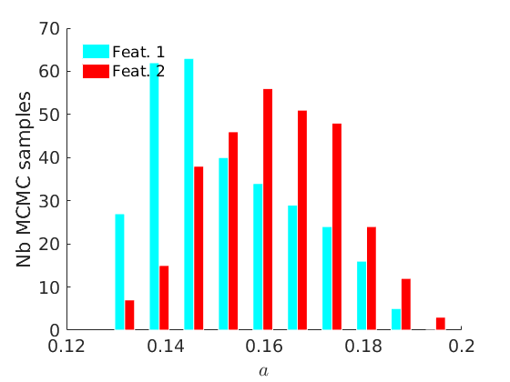
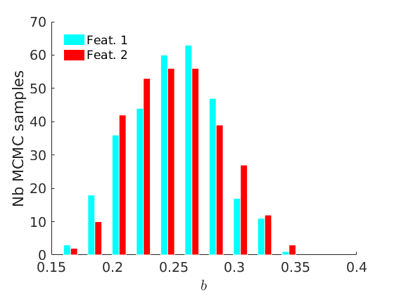
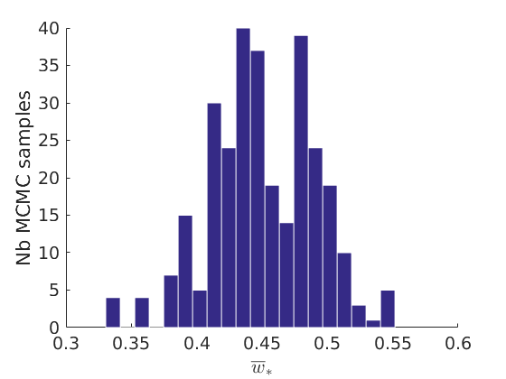
% Plot traces and histograms
variables = {'logalpha', 'sigma', 'tau', 'Fparam.a', 'Fparam.b', 'mean_w_rem'};
namesvar = {'$\log \alpha$', '$\sigma$', '$\tau$', '$a$', '$b$', '$\overline{w}_{\ast}$'};
plot_trace(objmcmc.samples, objmcmc.settings, variables, namesvar, [], outpath, prefix, suffix);
plot_hist(objmcmc.samples, variables, namesvar, [], ind_features, [], outpath, prefix, suffix);

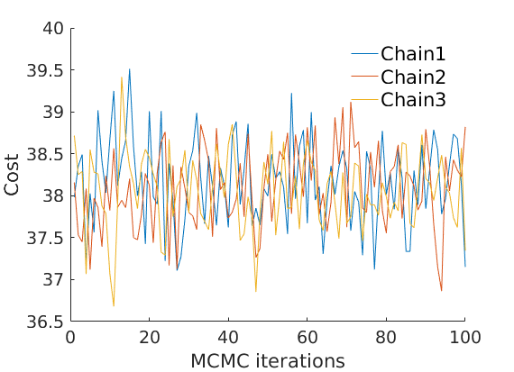
% Plot cost
if ~isempty(C_st)
    plot_cost(C_st, outpath, prefix, suffix);
end

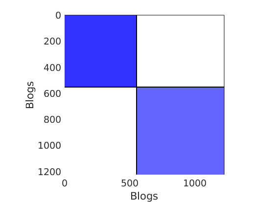
% Plot the graph by sorting the nodes by max feature to see block structure
plot_sortedgraph(G, nodefeat, nodefeat, ind_features, labels, outpath, prefix, suffix, {'png'});

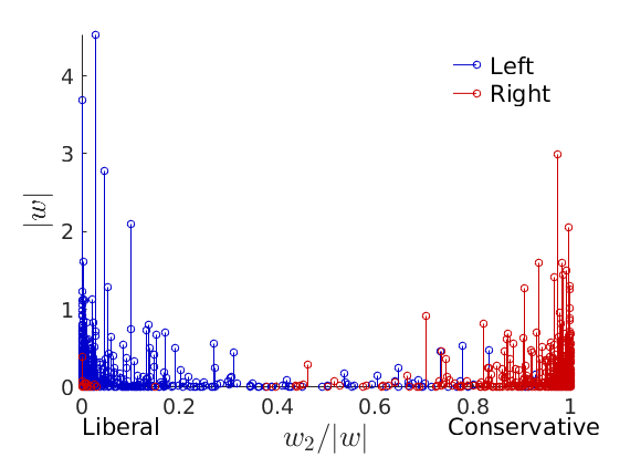
% Show the proportion in each features for a few nodes
if p==2
    color = color_groups;
elseif p==5
    color = [0 0 .5; .3 .3 1 ; 0.8 0.8 0.8 ; 1 .3 .3; .5 0 0];
end

if isfield(meta, 'groups')
    % Plots by groups right vs left
    plot_groups(estimates.w, meta.groups, meta.(groupfield), ind_features, label_groups, featnames, ...
        color_groups, outpath, prefix, suffix);

    y = sum(estimates.w,2);
    x = estimates.w(:,ind_features(2))./y;
    figure; hold on
    for i=1:numel(label_groups)
        ind = meta.groups==i;
        stem(x(ind), y(ind), 'o', 'markersize', 5, 'color', color(i,:))
    end
    xlabel('$w_{2}/\vert w \vert$', 'interpreter', 'latex', 'fontsize', 20)
    ylabel('$\vert w \vert$', 'interpreter', 'latex', 'fontsize', 20)
    text([0,.75], [-.5, -.5], featnames, 'fontsize', 16)
    legend(label_groups, 'fontsize', 16)
    legend boxoff
    axis tight
    xlim([0,1])
end

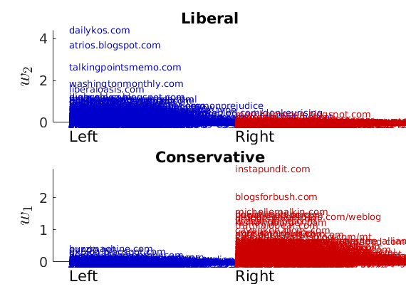
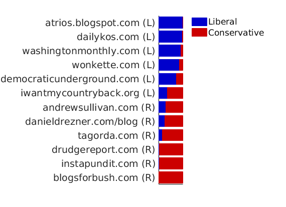
% Plot normalized weights for a subset of blogs
prop_nodes = estimates.w(:,1)./sum(estimates.w, 2);
names = {'blogsforbush.com'
    'instapundit.com'
    'drudgereport.com'
    'tagorda.com'
    'danieldrezner.com/blog'
    'andrewsullivan.com'
    'iwantmycountryback.org'
    'democraticunderground.com'
    'wonkette.com'
    'washingtonmonthly.com'
    'dailykos.com'
    'atrios.blogspot.com'};
ind = zeros(size(names,1),1);
lab = cell(size(names,1), 1);
for i=1:size(names,1)
    ind(i) = find(strcmp(meta.name, names{i}) & strcmp(meta.name, names{i,1}));
    lab{i} = sprintf('%s (%s)', names{i}, label_groups{meta.groups(ind(i))}(1));
%     fprintf('%2d. (%.2f) #%d, %s\n', i, prop_nodes(ind(i)), meta.degree{ind(i)}, lab{i});
end
plot_nodesfeatures(estimates.w, ind, ind_features, lab, featnames, color, outpath, prefix, suffix);

% Show blogs with highest weight in each feature
meta.wing = cell(meta.name);
meta.wing(meta.isright) = repmat({'R'}, sum(meta.isright), 1);
meta.wing(~meta.isright) = repmat({'L'}, sum(~meta.isright), 1);

fnames = {'degree', 'name', 'wing'};
formats = {'#%d,', '%s', '(%s).'}; %
% Nodes with highest weight in each feature
fprintf('-----------------------------------\n')
fprintf('Nodes with highest weights in each feature\n')
fprintf('#edges, name of blog (Political leaning)\n')
fprintf('-----------------------------------\n')
print_features( [outpath 'features_' num2str(p) 'f.txt'], ...
    estimates.w, ind_features, [], meta, fnames, formats );
fprintf('-----------------------------------\n')

-----------------------------------
Nodes with highest weights in each feature
#edges, name of blog (Political leaning)
-----------------------------------
& %--- FEATURE 1 ---
#351, dailykos.com (L). 
#277, atrios.blogspot.com (L). 
#274, talkingpointsmemo.com (L). 
#218, washingtonmonthly.com (L). 
#171, liberaloasis.com (L). 
#147, digbysblog.blogspot.com (L). 
#170, juancole.com (L). 
#149, newleftblogs.blogspot.com (L). 
#137, politicalstrategy.org (L). 
#144, pandagon.net (L). 
& %--- FEATURE 2 ---
#306, instapundit.com (R). 
#301, blogsforbush.com (R). 
#211, michellemalkin.com (R). 
#223, powerlineblog.com (R). 
#182, hughhewitt.com (R). 
#196, littlegreenfootballs.com/weblog (R). 
#243, drudgereport.com (R). 
#179, wizbangblog.com (R). 
#170, lashawnbarber.com (R). 
#199, truthlaidbear.com (R). 
-----------------------------------

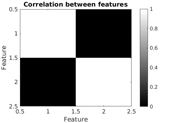
% Correlation between the features
figure('name', 'Correlation between features');
imagesc(corr(estimates.w(:,ind_features)));
colormap('gray')
caxis([0,1])
colorbar
xlabel('Feature')
ylabel('Feature')
title('Correlation between features')

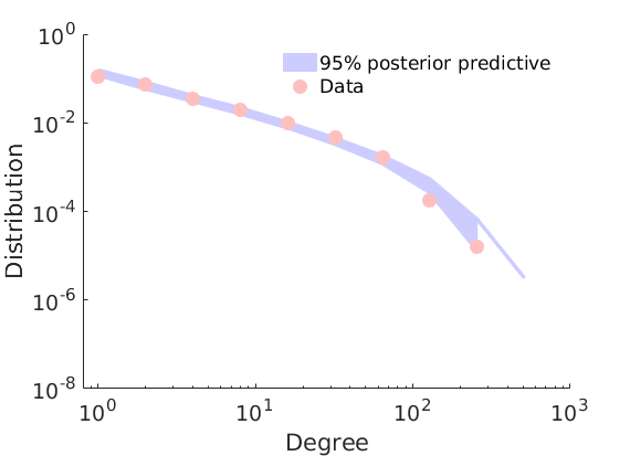
% Plot posterior predictive of degree distribution
plot_degreepostpred(G, objmcmc, nsamples, 1e-6, outpath, prefix, suffix);

-----------------------------------
Start degree posterior predictive estimation: 100 draws
Estimated end of computation: 08-Nov-2017 18:04:16 (0.0 hours)
|---------------------------------|
|*********************************|
End degree posterior predictive (0.0 hours)
-----------------------------------

Sparse Networks with Overlapping Communities (SNetOC) package: demo_polblogs

Contents

General settings

Load network of political blogs

Posterior Inference using Markov chain Monte Carlo and point estimation

Plots