Sparse Networks with Overlapping Communities (SNetOC) package: demo_usairport

This Matlab script performs posterior inference on a network of airports to find latent overlapping communities, using a Bayesian nonparametric approach.

For downloading the package and information on installation, visit the SNetOC webpage.

Reference:

A. Todeschini, X. Miscouridou and F. Caron (2017) Exchangeable Random Measures for Sparse and Modular Graphs with Overlapping Communities. arXiv:1602.02114.

Authors:

A. Todeschini, Inria
X. Miscouridou, University of Oxford
F. Caron, University of Oxford

Tested on Matlab R2016a. Requires the Statistics toolbox.

Last Modified: 10/10/2017

General settings
Load Network of airports with a connection to a US airport
Posterior Inference using Markov chain Monte Carlo and point estimation
Plots

General settings

clear
close all
tstart = clock; % Starting time

istest = true; % enable testing mode: quick run with smaller nb of iterations

In test mode, a smaller number of iterations is run. Although the sampler clearly has not converged yet, the method already recovers well interpretable latent communities. To reproduce the results of the paper, set this value to false.

root = '.';
if istest
    outpath = fullfile(root, 'results', 'demo_usairport', 'test');
else
    outpath = fullfile(root, 'results', 'demo_usairport', date);
end

if ~isdir(outpath)
    mkdir(outpath);
end


% Add path
addpath ./GGP/ ./CGGP/ ./utils/

% Default fontsize
set(0, 'DefaultAxesFontSize', 14)

% Set the seed
rng default

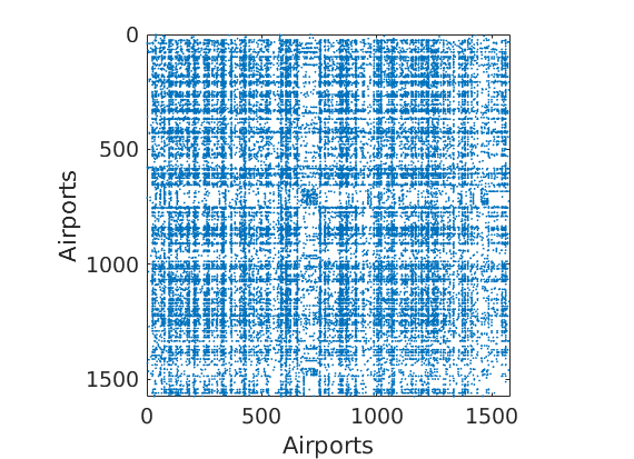
Load Network of airports with a connection to a US airport

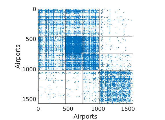
load ./data/usairport/usairport

titlenetwork = 'US airport network in 2010';
name = 'usairport';
labels = {'Airports','Airports'};

G = G | G'; % make undirected graph
G = logical(G-diag(diag(G))); % remove self edges (#164)

meta.degree = num2cell(full(sum(G,2)));
fn = fieldnames(meta);

% Plot adjacency matrix
figure
spy(G);
xlabel(labels{2})
ylabel(labels{1})

Posterior Inference using Markov chain Monte Carlo and point estimation

Users needs to start the parallel pool by using the command parpool to run multiple chains in parallel.

% Define the parameters of the prior
p = 4; % Number of commmunities
objprior =  graphmodel('CGGP', p); % CGGP graph model with p communities

% Define parameters of the MCMC sampler
nchains = 3;
if istest
    niterinit = 1000;
    niter = 20000;
    nsamples = 100;
else
    niterinit = 10000;
    niter = 200000;
    nsamples = 500;
end
nburn = floor(niter/2);
thin = ceil((niter-nburn)/nsamples);
verbose = true;

% Create the graphMCMC object
objmcmc = graphmcmc(objprior, niter, nburn, thin, nchains);

% Run initialisation
init = graphinit(objmcmc, G, niterinit);

-----------------------------------
Start initialisation of the MCMC algorithm for CGGP
-----------------------------------
End initialisation
-----------------------------------

% Run MCMC sampler
objmcmc = graphmcmcsamples(objmcmc, G, verbose, init);

-----------------------------------
Start MCMC for CGGP graphs
Nb of nodes: 1574 - Nb of edges: 17215 (0 missing)
Nb of chains: 3 - Nb of iterations: 20000
Nb of parallel workers: 1
Estimated computation time: 0 hour(s) 6 minute(s)
Estimated end of computation: 08-Nov-2017 18:16:42 
-----------------------------------
 Markov chain 1/3 
-----------------------------------
i=2000 alp=110.74 sig=0.214 tau=0.99 a=0.31 0.36 0.17 0.32 b=0.47 0.30 0.03 0.42 w*=0.41 0.66 1.36 0.39 b2=0.47 0.29 0.03 0.41 alp2=110.38 rhmc=0.65 rhyp=0.24 eps=0.015 rwsd=0.027
i=4000 alp=112.25 sig=0.191 tau=1.28 a=0.26 0.29 0.14 0.28 b=0.24 0.16 0.01 0.25 w*=0.39 0.64 1.49 0.43 b2=0.31 0.20 0.02 0.32 alp2=117.72 rhmc=0.56 rhyp=0.23 eps=0.044 rwsd=0.027
i=6000 alp=109.62 sig=0.196 tau=1.44 a=0.26 0.28 0.12 0.25 b=0.22 0.15 0.01 0.22 w*=0.44 0.63 1.27 0.41 b2=0.32 0.21 0.01 0.32 alp2=117.69 rhmc=0.71 rhyp=0.25 eps=0.011 rwsd=0.027
i=8000 alp=111.37 sig=0.184 tau=1.70 a=0.24 0.28 0.11 0.27 b=0.18 0.11 0.01 0.18 w*=0.35 0.62 1.34 0.37 b2=0.31 0.19 0.01 0.30 alp2=122.79 rhmc=0.92 rhyp=0.25 eps=0.011 rwsd=0.027
i=10000 alp=88.97 sig=0.218 tau=1.95 a=0.24 0.25 0.11 0.24 b=0.16 0.10 0.01 0.15 w*=0.39 0.72 1.46 0.47 b2=0.31 0.19 0.01 0.29 alp2=102.86 rhmc=0.92 rhyp=0.25 eps=0.011 rwsd=0.027
i=12000 alp=94.45 sig=0.208 tau=1.99 a=0.24 0.24 0.10 0.23 b=0.16 0.08 0.01 0.14 w*=0.38 0.72 1.39 0.40 b2=0.32 0.15 0.01 0.28 alp2=108.99 rhmc=0.92 rhyp=0.27 eps=0.011 rwsd=0.027
i=14000 alp=93.23 sig=0.212 tau=1.94 a=0.23 0.22 0.10 0.23 b=0.15 0.07 0.01 0.12 w*=0.39 0.70 1.45 0.41 b2=0.29 0.13 0.01 0.23 alp2=107.33 rhmc=0.92 rhyp=0.26 eps=0.011 rwsd=0.027
i=16000 alp=77.03 sig=0.235 tau=1.65 a=0.22 0.24 0.10 0.22 b=0.13 0.07 0.00 0.11 w*=0.39 0.71 1.52 0.40 b2=0.22 0.11 0.01 0.18 alp2=86.67 rhmc=0.92 rhyp=0.26 eps=0.011 rwsd=0.027
i=18000 alp=86.39 sig=0.218 tau=2.16 a=0.22 0.23 0.10 0.22 b=0.11 0.06 0.00 0.10 w*=0.40 0.66 1.52 0.42 b2=0.23 0.14 0.01 0.22 alp2=102.16 rhmc=0.92 rhyp=0.26 eps=0.011 rwsd=0.027
i=20000 alp=91.88 sig=0.216 tau=2.72 a=0.20 0.21 0.10 0.21 b=0.08 0.05 0.00 0.10 w*=0.48 0.66 1.33 0.37 b2=0.21 0.13 0.01 0.26 alp2=113.97 rhmc=0.92 rhyp=0.28 eps=0.011 rwsd=0.027
-----------------------------------
 Markov chain 2/3 
-----------------------------------
i=2000 alp=106.28 sig=0.220 tau=0.89 a=0.46 0.45 0.18 0.32 b=0.49 0.78 0.03 0.40 w*=0.66 0.40 1.65 0.44 b2=0.43 0.69 0.02 0.35 alp2=103.52 rhmc=0.67 rhyp=0.25 eps=0.016 rwsd=0.027
i=4000 alp=99.13 sig=0.217 tau=1.12 a=0.35 0.34 0.13 0.27 b=0.24 0.38 0.01 0.26 w*=0.64 0.35 1.77 0.36 b2=0.26 0.43 0.01 0.29 alp2=101.60 rhmc=0.52 rhyp=0.23 eps=0.035 rwsd=0.028
i=6000 alp=97.90 sig=0.219 tau=1.49 a=0.30 0.29 0.12 0.24 b=0.14 0.24 0.01 0.22 w*=0.64 0.45 1.60 0.40 b2=0.21 0.36 0.01 0.33 alp2=106.92 rhmc=0.81 rhyp=0.24 eps=0.011 rwsd=0.027
i=8000 alp=99.78 sig=0.214 tau=1.36 a=0.30 0.26 0.12 0.23 b=0.13 0.19 0.01 0.17 w*=0.71 0.39 1.46 0.40 b2=0.17 0.26 0.01 0.24 alp2=106.52 rhmc=0.93 rhyp=0.23 eps=0.011 rwsd=0.027
i=10000 alp=88.70 sig=0.218 tau=1.44 a=0.26 0.26 0.11 0.23 b=0.08 0.16 0.00 0.17 w*=0.65 0.41 1.81 0.37 b2=0.12 0.23 0.01 0.24 alp2=95.99 rhmc=0.93 rhyp=0.25 eps=0.011 rwsd=0.027
i=12000 alp=87.79 sig=0.223 tau=1.83 a=0.28 0.26 0.10 0.23 b=0.10 0.16 0.00 0.14 w*=0.62 0.45 1.69 0.40 b2=0.19 0.28 0.01 0.25 alp2=100.45 rhmc=0.93 rhyp=0.26 eps=0.011 rwsd=0.027
i=14000 alp=92.23 sig=0.206 tau=1.87 a=0.27 0.26 0.10 0.22 b=0.09 0.15 0.00 0.12 w*=0.60 0.41 1.53 0.39 b2=0.17 0.28 0.01 0.23 alp2=104.97 rhmc=0.93 rhyp=0.24 eps=0.011 rwsd=0.027
i=16000 alp=92.20 sig=0.217 tau=2.13 a=0.24 0.26 0.10 0.21 b=0.06 0.15 0.00 0.09 w*=0.78 0.43 1.45 0.46 b2=0.12 0.32 0.01 0.20 alp2=108.64 rhmc=0.93 rhyp=0.25 eps=0.011 rwsd=0.027
i=18000 alp=83.51 sig=0.226 tau=1.84 a=0.25 0.24 0.10 0.21 b=0.07 0.11 0.00 0.11 w*=0.74 0.45 1.64 0.44 b2=0.13 0.21 0.01 0.21 alp2=95.91 rhmc=0.93 rhyp=0.24 eps=0.011 rwsd=0.027
i=20000 alp=78.20 sig=0.226 tau=1.77 a=0.22 0.24 0.10 0.19 b=0.04 0.11 0.00 0.07 w*=0.72 0.41 1.30 0.40 b2=0.08 0.20 0.01 0.13 alp2=88.92 rhmc=0.93 rhyp=0.24 eps=0.011 rwsd=0.027
-----------------------------------
 Markov chain 3/3 
-----------------------------------
i=2000 alp=150.61 sig=0.161 tau=1.51 a=0.26 0.34 0.24 0.27 b=0.13 0.60 0.11 0.24 w*=0.98 0.56 0.67 0.51 b2=0.20 0.91 0.16 0.36 alp2=160.94 rhmc=0.65 rhyp=0.25 eps=0.016 rwsd=0.028
i=4000 alp=132.48 sig=0.172 tau=2.05 a=0.20 0.26 0.21 0.22 b=0.06 0.35 0.06 0.10 w*=1.28 0.49 0.65 0.47 b2=0.12 0.71 0.12 0.21 alp2=149.90 rhmc=0.60 rhyp=0.24 eps=0.038 rwsd=0.029
i=6000 alp=160.23 sig=0.144 tau=3.05 a=0.18 0.24 0.19 0.18 b=0.05 0.34 0.05 0.08 w*=1.20 0.52 0.55 0.55 b2=0.14 1.02 0.16 0.24 alp2=188.05 rhmc=0.70 rhyp=0.24 eps=0.014 rwsd=0.029
i=8000 alp=143.54 sig=0.153 tau=4.12 a=0.18 0.23 0.17 0.18 b=0.05 0.26 0.04 0.05 w*=1.12 0.55 0.61 0.49 b2=0.20 1.07 0.16 0.22 alp2=178.31 rhmc=0.88 rhyp=0.23 eps=0.014 rwsd=0.029
i=10000 alp=152.81 sig=0.153 tau=4.38 a=0.17 0.23 0.17 0.16 b=0.04 0.25 0.04 0.05 w*=1.32 0.52 0.62 0.64 b2=0.17 1.10 0.17 0.20 alp2=191.44 rhmc=0.89 rhyp=0.24 eps=0.014 rwsd=0.029
i=12000 alp=150.76 sig=0.146 tau=4.83 a=0.16 0.22 0.16 0.16 b=0.04 0.25 0.03 0.04 w*=1.02 0.53 0.69 0.62 b2=0.18 1.20 0.15 0.20 alp2=189.79 rhmc=0.88 rhyp=0.24 eps=0.014 rwsd=0.029
i=14000 alp=179.23 sig=0.117 tau=7.53 a=0.16 0.20 0.15 0.16 b=0.03 0.17 0.03 0.04 w*=1.24 0.56 0.65 0.48 b2=0.22 1.31 0.21 0.28 alp2=226.94 rhmc=0.88 rhyp=0.24 eps=0.014 rwsd=0.029
i=16000 alp=224.15 sig=0.083 tau=8.27 a=0.16 0.20 0.14 0.15 b=0.04 0.17 0.03 0.03 w*=1.02 0.45 0.51 0.56 b2=0.29 1.38 0.21 0.24 alp2=267.00 rhmc=0.88 rhyp=0.25 eps=0.014 rwsd=0.029
i=18000 alp=204.00 sig=0.092 tau=8.33 a=0.16 0.18 0.13 0.15 b=0.03 0.15 0.02 0.03 w*=1.08 0.60 0.59 0.52 b2=0.26 1.21 0.14 0.21 alp2=247.76 rhmc=0.88 rhyp=0.25 eps=0.014 rwsd=0.029
i=20000 alp=181.18 sig=0.116 tau=9.41 a=0.15 0.18 0.13 0.14 b=0.03 0.12 0.02 0.02 w*=0.97 0.52 0.59 0.63 b2=0.26 1.15 0.16 0.23 alp2=234.88 rhmc=0.88 rhyp=0.23 eps=0.014 rwsd=0.029
-----------------------------------
End MCMC
Computation time: 0 hour(s) 6 minute(s)
-----------------------------------

% Print summary in text file
print_summary(['summary_' num2str(p) 'f.txt'], titlenetwork, G, niter, nburn, nchains, thin, p, outpath, tstart)

% Point estimation of the model parameters
[estimates, C_st] = graphest(objmcmc);

% Save workspace
save(fullfile(outpath, ['workspace_' num2str(p) 'f.mat']))

-----------------------------------
Start parameters estimation for CGGP graphs: 300 samples
Estimated end of computation: 08-Nov-2017 18:17:36 (0.0 hours)
|---------------------------------|
|*********************************|
End parameters estimation for CGGP graphs
Computation time: 0.0 hours
-----------------------------------

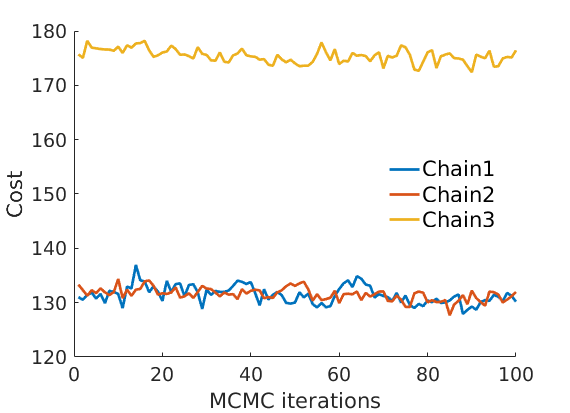
Plots

prefix = sprintf('%s_%df_', name, p);
suffix = '';

% Plot cost
if ~isempty(C_st)
    plot_cost(C_st, outpath, prefix, suffix);
end
% Assign max feature for community detection
[~, nodefeat] = max(estimates.w, [],2);

% Identify each feature/community as Hub/East/West/Alaska
% (This step would normally require a human interpretation of the features)
code_airports = {'JFK', 'LAN', 'DEN', 'BET'};
for k=1:length(code_airports)
    [~, ind_features(k)] = max(estimates.w(strcmp(meta.code, code_airports{k}), :));
end
if length(unique(ind_features))~=4
    warning('Problem with the interpretation of features/communities');
    ind_features = 1:4;
    featnames = {'Feature 1', 'Feature 2', 'Feature 3', 'Feature 4'};
else
    featnames = {'Hub', 'East', 'West', 'Alaska'};
end

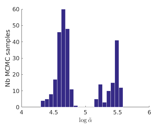
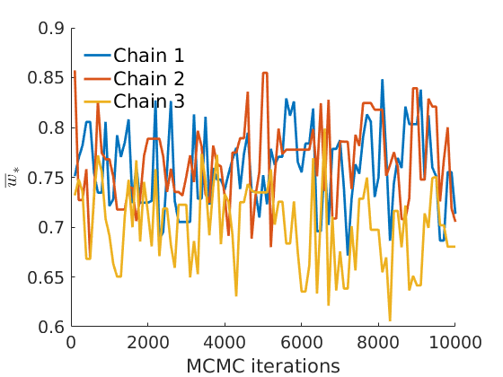
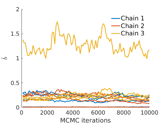
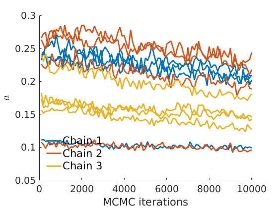
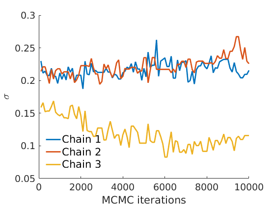
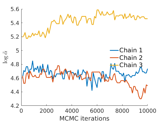
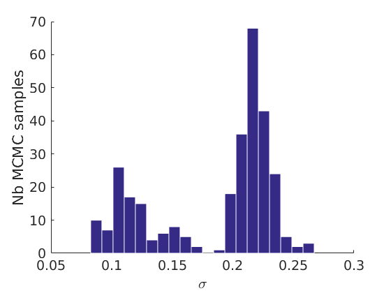
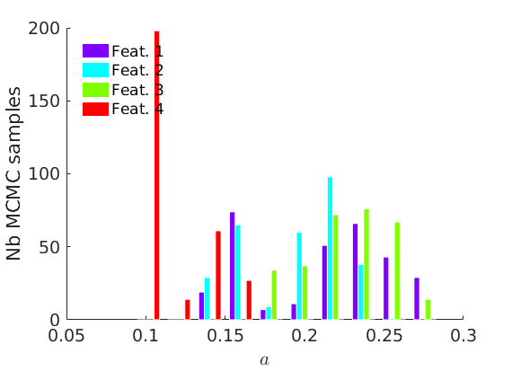
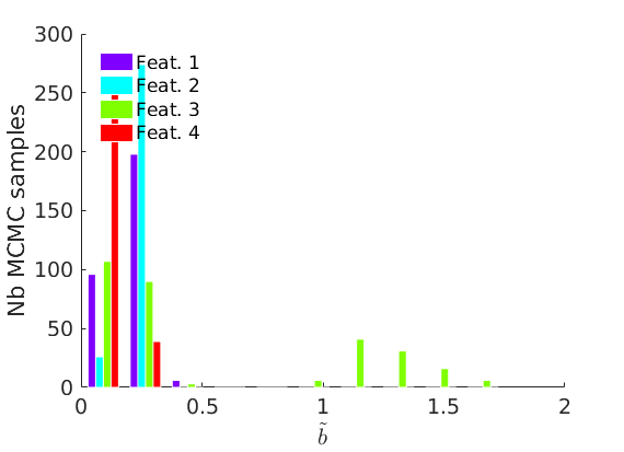
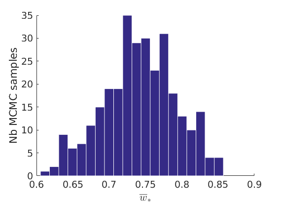
% Plot traces and histograms
variables = {'logalpha2', 'sigma', 'Fparam.a', 'Fparam.b2', 'mean_w_rem'};
namesvar = {'$\log \tilde\alpha$', '$\sigma$', '$a$', '$\tilde b$', '$\overline{w}_{\ast}$'};
plot_trace(objmcmc.samples, objmcmc.settings, variables, namesvar, [], outpath, prefix, suffix);
plot_hist(objmcmc.samples, variables, namesvar, [], ind_features, [], outpath, prefix, suffix);

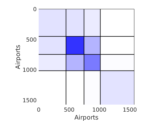
% Plot the graph by sorting the nodes by max feature
plot_sortedgraph(G, nodefeat, nodefeat, ind_features, labels, outpath, prefix, suffix, {'png'});

if isfield(meta, 'groups')
    % Plots by groups right vs left
    plot_groups(estimates.w, meta.groups, meta.(groupfield), ind_features, label_groups, featnames, color_groups, outpath, prefix, suffix);
end

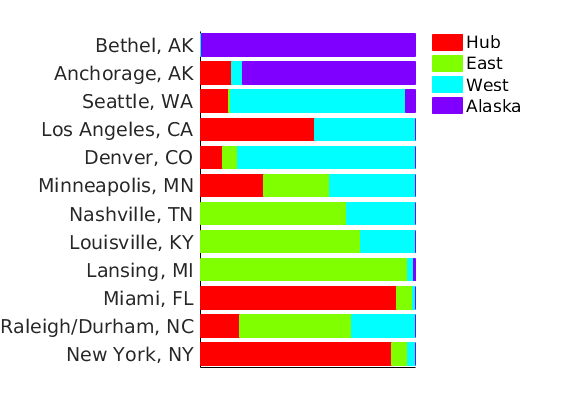
% Show the proportion in each features for a few nodes
% https://www.mapcustomizer.com/
names = {
    'New York, NY'
%     'Washington, DC'
    'Miami, FL'
%     'Detroit, MI'
%     'Knoxville, TN'
%     'Atlanta, GA'
%     'Louisville, KY'
%     'Indianapolis, IN'
    'Raleigh/Durham, NC'
    'Nashville, TN'
%     'Chicago, IL'
%     'Fayetteville, NC'
    'Lansing, MI'
    'Louisville, KY'
%     'Memphis, TN'
%     'Cleveland, OH'
    'Minneapolis, MN'
%     'Charleston/Dunbar, WV'
%     'Baltimore, ML'
%     'Tallahassee, FL'
%     'Portland, ME'
%     'Flint, MI'
%     'Champaign/Urbana, IL'
%     'Oklahoma City, OK'
%     'Des Moines, IA'
%     'Houston, TX'
%     'Dallas, TX'
    'Denver, CO'
%     'Fort Wayne, IN'
%     'Tyler, TX'
%     'Salt Lake City, UT'
%     'Phoenix, AZ'
    'Los Angeles, CA'
    'Seattle, WA'
%     'San Francisco, CA'
%     'Fairbanks, AK'
    'Anchorage, AK'
    'Bethel, AK'
};
ind = zeros(size(names,1),1);
for i=1:size(names,1)
    I = find(strcmp(meta.city, names{i}));
    [~, imax] = max([meta.degree{I}]);
    ind(i) = I(imax);
end
[~, ind2] = sort(meta.lon(ind), 'descend');
ind = ind(ind2);
names = names(ind2);
color = hsv(p);
plot_nodesfeatures(estimates.w, ind, ind_features, names, featnames, color, outpath, prefix, suffix);

% Show some of the nodes in each feature
fnames = {'degree', 'city'}; % meta fields displayed for features exploration
formats = {'#%d,', '%s.'}; %
print_features( fullfile(outpath, ['features_' num2str(p) 'f.txt']), ...
    estimates.w, ind_features, featnames, meta, fnames, formats)
print_features( fullfile(outpath, ['featuresnorm_' num2str(p) 'f.txt']), ...
    bsxfun(@rdivide, estimates.w, sum(estimates.w,2)),...
    ind_features, featnames, meta, fnames, formats)

fnames = {'city'}; % meta fields displayed for features exploration
formats = {'%s.'}; %
print_features( fullfile(outpath, ['features_' num2str(p) 'f_tex.txt']), ...
    estimates.w, ind_features, featnames, meta, fnames, formats)
print_features( fullfile(outpath, ['featuresnorm_' num2str(p) 'f_tex.txt']), ...
    bsxfun(@rdivide, estimates.w, sum(estimates.w,2)),...
    ind_features, featnames, meta, fnames, formats)

& %--- Hub ---
#291, New York, NY. 
#299, Washington, DC. 
#261, Miami, FL. 
#245, Boston, MA. 
#292, Los Angeles, CA. 
#273, Newark, NJ. 
#314, Atlanta, GA. 
#211, Fort Lauderdale, FL. 
#231, Orlando, FL. 
#244, Philadelphia, PA. 
& %--- East ---
#296, Chicago, IL. 
#252, Detroit, MI. 
#314, Atlanta, GA. 
#204, Nashville, TN. 
#184, Indianapolis, IN. 
#203, Cleveland, OH. 
#195, Pittsburgh, PA. 
#173, Louisville, KY. 
#299, Washington, DC. 
#189, Memphis, TN. 
& %--- West ---
#274, Denver, CO. 
#240, Las Vegas, NV. 
#219, Burbank, CA. 
#292, Los Angeles, CA. 
#183, Salt Lake City, UT. 
#214, San Francisco, CA. 
#190, Phoenix, AZ. 
#193, Seattle, WA. 
#254, Dallas/Fort Worth, TX. 
#267, Houston, TX. 
& %--- Alaska ---
#172, Anchorage, AK. 
#131, Fairbanks, AK. 
#83, Bethel, AK. 
#37, Iliamna, AK. 
#60, King Salmon, AK. 
#48, St. Mary's, AK. 
#49, McGrath, AK. 
#47, Dillingham, AK. 
#49, Galena, AK. 
#44, Kotzebue, AK. 
& %--- Hub ---
#3, Johnstown, PA. 
#1, Sarajevo, Yugoslavia. 
#2, Oneonta, NY. 
#1, Ahmedabad, India. 
#3, Pittsfield, MA. 
#37, Charlotte Amalie, Virgin Islands. 
#1, Palermo, Italy. 
#3, La Romana, Dominican Republic. 
#1, Casablanca, Morocco. 
#3, Barrancabermeja, Colombia. 
& %--- East ---
#70, Daytona Beach, FL. 
#22, Binghamton, NY. 
#75, Pensacola, FL. 
#46, Newport News/Williamsburg, VA. 
#30, London, Canada. 
#51, Kalamazoo, MI. 
#51, Fayetteville, NC. 
#50, Scranton/Wilkes-Barre, PA. 
#4, Cape Girardeau, MO. 
#3, Williamsport, PA. 
& %--- West ---
#9, Leon/Guanajuato, Mexico. 
#51, Kalispell, MT. 
#20, Durango, CO. 
#3, Santa Cruz/Huatulco, Mexico. 
#1, Philadelphia, PA. 
#136, Reno, NV. 
#3, Battle Creek, MI. 
#30, Medford, OR. 
#76, Lubbock, TX. 
#16, San Luis Obispo, CA. 
& %--- Alaska ---
#4, Cape Newenham, AK. 
#21, Napakiak, AK. 
#4, Majuro, Marshall Islands District (TTPI). 
#24, Alakanuk, AK. 
#8, Hoolehua, HI. 
#1, Dunbar, Australia. 
#17, Sheldon Point, AK. 
#27, Kalskag, AK. 
#2, Seward, AK. 
#23, Kwigillingok, AK. 
& %--- Hub ---
New York, NY. 
Washington, DC. 
Miami, FL. 
Boston, MA. 
Los Angeles, CA. 
Newark, NJ. 
Atlanta, GA. 
Fort Lauderdale, FL. 
Orlando, FL. 
Philadelphia, PA. 
& %--- East ---
Chicago, IL. 
Detroit, MI. 
Atlanta, GA. 
Nashville, TN. 
Indianapolis, IN. 
Cleveland, OH. 
Pittsburgh, PA. 
Louisville, KY. 
Washington, DC. 
Memphis, TN. 
& %--- West ---
Denver, CO. 
Las Vegas, NV. 
Burbank, CA. 
Los Angeles, CA. 
Salt Lake City, UT. 
San Francisco, CA. 
Phoenix, AZ. 
Seattle, WA. 
Dallas/Fort Worth, TX. 
Houston, TX. 
& %--- Alaska ---
Anchorage, AK. 
Fairbanks, AK. 
Bethel, AK. 
Iliamna, AK. 
King Salmon, AK. 
St. Mary's, AK. 
McGrath, AK. 
Dillingham, AK. 
Galena, AK. 
Kotzebue, AK. 
& %--- Hub ---
Johnstown, PA. 
Sarajevo, Yugoslavia. 
Oneonta, NY. 
Ahmedabad, India. 
Pittsfield, MA. 
Charlotte Amalie, Virgin Islands. 
Palermo, Italy. 
La Romana, Dominican Republic. 
Casablanca, Morocco. 
Barrancabermeja, Colombia. 
& %--- East ---
Daytona Beach, FL. 
Binghamton, NY. 
Pensacola, FL. 
Newport News/Williamsburg, VA. 
London, Canada. 
Kalamazoo, MI. 
Fayetteville, NC. 
Scranton/Wilkes-Barre, PA. 
Cape Girardeau, MO. 
Williamsport, PA. 
& %--- West ---
Leon/Guanajuato, Mexico. 
Kalispell, MT. 
Durango, CO. 
Santa Cruz/Huatulco, Mexico. 
Philadelphia, PA. 
Reno, NV. 
Battle Creek, MI. 
Medford, OR. 
Lubbock, TX. 
San Luis Obispo, CA. 
& %--- Alaska ---
Cape Newenham, AK. 
Napakiak, AK. 
Majuro, Marshall Islands District (TTPI). 
Alakanuk, AK. 
Hoolehua, HI. 
Dunbar, Australia. 
Sheldon Point, AK. 
Kalskag, AK. 
Seward, AK. 
Kwigillingok, AK.

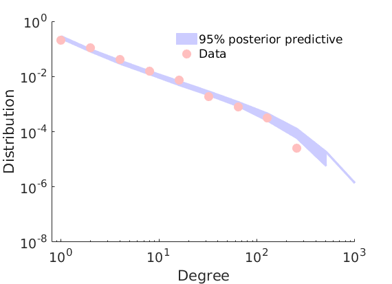
 % Plot posterior predictive of degrees
 plot_degreepostpred(G, objmcmc, nsamples, 1e-6, outpath, prefix, suffix);

-----------------------------------
Start degree posterior predictive estimation: 100 draws
Estimated end of computation: 08-Nov-2017 18:18:07 (0.0 hours)
|---------------------------------|
|*********************************|
End degree posterior predictive (0.0 hours)
-----------------------------------

Sparse Networks with Overlapping Communities (SNetOC) package: demo_usairport

Contents

General settings

Load Network of airports with a connection to a US airport

Posterior Inference using Markov chain Monte Carlo and point estimation

Plots